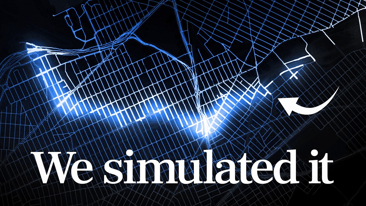
No clickbait detected — the title and thumbnail deliver what they promise.
AI Opinion
The episode convincingly argues that Google Maps achieves its speed by pre-computing node importance in the road network, using graph cuts like the 102 Mississippi River bridges to dramatically shrink the search space for long routes. Its strongest verified claims—such as Dijkstra’s 1956 origin and the impracticality of a full lookup table—are well-supported, but the staggering figures of 64 million intersections and 10^220 possible routes are labeled "Needs Research" and should be treated as illustrative estimates rather than precise facts. A thoughtful viewer should verify whether the "bridge nodes" concept truly scales to all regions and road types, as the episode’s neat example may oversimplify the complexity of real-world routing across diverse terrains.
Voices are AI rewrites of the same facts — style changes, not substance.
Summary
The episode explains how Google Maps achieves remarkably fast route calculations despite the astronomical scale of the problem—the North American road network has over 64 million intersections, with roughly 10^220 possible routes from New York to San Francisco. It traces the origin of Dijkstra's algorithm, conceived by Edsger Dijkstra in 1956 during a shopping trip in Amsterdam, which efficiently finds the shortest path by always exploring the nearest unvisited node. Early GPS systems in the 1990s used manually annotated road hierarchies to run a bi-directional Dijkstra that prioritized major roads, reducing the search area. Google Maps improves on this by automatically pre-processing the graph to order nodes by importance, measured by how many shortest paths include them. For example, a bridge connecting two towns becomes more important as the towns grow, and a small set of nodes that splits the graph—such as 102 bridges over the Mississippi River in the North American network—receives the highest rank, as any coast-to-coast trip must pass through one. The episode also highlights the trade-off between preprocessing and query runtime: a massive lookup table of all shortest paths would require over a decade of compute and more than eight petabytes of data, while being brittle to road changes. Google Maps strikes a middle ground, achieving very fast queries with moderate preprocessing.
Voices are AI rewrites of the same facts — style changes, not substance.
Key Points
Scale of the Shortest Path Problem
The North American road system has over 64 million intersections, yielding roughly 10^220 possible routes from New York to San Francisco. Even checking a billion routes per second would take over 10^200 years, yet Google Maps finds a route in about four seconds. This highlights the need for efficient algorithms, not brute force.
Origin of Dijkstra's Algorithm
In 1956, Edsger Dijkstra was developing software for the ARMAC computer in the Netherlands. To demonstrate the computer's power to a skeptical public, he needed a problem non-mathematicians could understand. During a shopping trip in Amsterdam with his fiancée, he conceived the shortest path problem: 'What's the shortest way to travel from Rotterdam to Groningen?' This led to the creation of Dijkstra's algorithm.
Breadth-First Search Limitations
The simplest shortest path algorithm, Breadth-First Search (BFS), explores all nodes one step away, then two steps, etc., until the destination is found. However, BFS treats all roads as equal length, which is unrealistic. In a weighted graph (where edges have distances), BFS fails because it doesn't account for varying edge weights, making it unsuitable for real-world navigation.
Dijkstra's Algorithm Mechanics
Dijkstra's algorithm maintains a 'cost' (shortest known distance) for each node, starting at zero for the source and infinity for others. It repeatedly explores the unexplored node with the lowest cost, updating neighbor costs if a shorter path is found. For example, from Rotterdam, it updates neighbors to costs 1, 2, 3, and 4, then explores the node with cost 2 next. The algorithm continues until all nodes are explored, ensuring the first time it reaches the goal, it has the true shortest path.
Road hierarchy encoding in early GPS systems
In the 1990s, early in-car GPS systems used pre-computed road classes annotated on roads. Surveyors manually recorded road attributes like speed limit, width, and highway status, which mapping companies then categorized into hierarchies such as express highway, local major road, or narrow road. The GPS ran a bi-directional Dijkstra algorithm that first searched narrow roads within a candidate area, then moved up to major local roads, and finally to highways if needed, reducing the search area by leveraging the hierarchy.
Trade-off between preprocessing and query runtime
A massive lookup table of all shortest paths would give insanely fast query runtimes but requires over a decade of compute on a single core and more than eight petabytes of raw data—equivalent to storing Wikipedia 16 times over. Additionally, any road closure or new bridge would require rebuilding large portions. In contrast, Dijkstra's algorithm needs no preprocessing but takes a long time to run. Google Maps aims for a middle ground: very fast query runtimes with moderate preprocessing.
Automatic node importance ordering
Instead of manual hierarchies, Google Maps automatically pre-processes the graph to order nodes by importance. For example, an exit connecting two highways is highly important, while a cul-de-sac intersection is not. This allows a bi-directional Dijkstra that searches up the hierarchy from both directions, eliminating the need for candidate areas while still guaranteeing the shortest path.
Bridge nodes and graph cuts determine importance
Node importance is measured by how many shortest paths include it. A bridge connecting two towns becomes more important as more houses are added on either side, peaking when the towns are roughly equal size and the bridge splits the graph in half. A small set of nodes that splits the graph—like 102 nodes along the Mississippi River in the North American network—gets the highest rank, as any trip from east to west coast must pass through one of them.
Chapters
Claims & Fact Check
There are over 64 million intersections in the North American road system.
?UnverifiedA simplified estimate gives around 10 to the 220 possible routes from New York to San Francisco.
?UnverifiedDijkstra's algorithm was conceived during a shopping trip in Amsterdam in 1956.
?UnverifiedBuilding a massive lookup table of all shortest paths from every intersection would take more than a decade of compute on a single core and require over eight petabytes of raw data.
?UnverifiedA small set of nodes that splits the graph in half is important because the maximum number of shortest paths include that set.
?UnverifiedThe 102 blue nodes that roughly split the North American graph in half correspond to bridges over the Mississippi River.
?Unverified